Questions may be directed to resonate@ekkobit.com

Theory¶

In the following text — and in the code —, we adopt the convention that window means a number of previous data points + the current data point. n_sma, n_ema etc. and the number in EMA3, L14, H14 etc. is the window — the current data point, i.e only previous data points. The distinction is important in order avoid confusion.

Trend-following Indicators¶

Trend-following indicators are lagging indicators, which means they change only after the market change. They do their best work when markets are moving up or down and become unreliable when markets flatten out.

Simple Moving Average (SMA)¶

To find the simple moving average at time \(t\), take a data point at time \(t\) - add to it a certain number of past data points - and divide by the total number of data points. In the following, let’s say our data points are stock prices.

\[\text{sma}_t = \dfrac{\sum\limits_{i=0}^{n} \text{price}_{(t-i)}}{n + 1}\]

\(sma_t\): simple moving average calculated for time \(t\)
\(\text{price}_{(t-i)}\): Current and previous prices in sma
\(n\): Number of previous prices to include in calculation. Total number of prices is \(n + 1\)

Let’s set \(n = 3\), which means we include 3 previous prices in the sma. Now, we can’t start at \(t=0\), because we need at least 3 previous prices. At the earliest, we can start at \(t=3\), provided there is such a thing as \(t=0\). So let’s expand the formula. At \(t=3\). What we get is this:

\[\text{sma}_{t=3} = \dfrac{p_{(t=3)} + p_{(t=2)} + p_{(t=1)} + p_{(t=0)}}{4},\]

\(p\): short for price

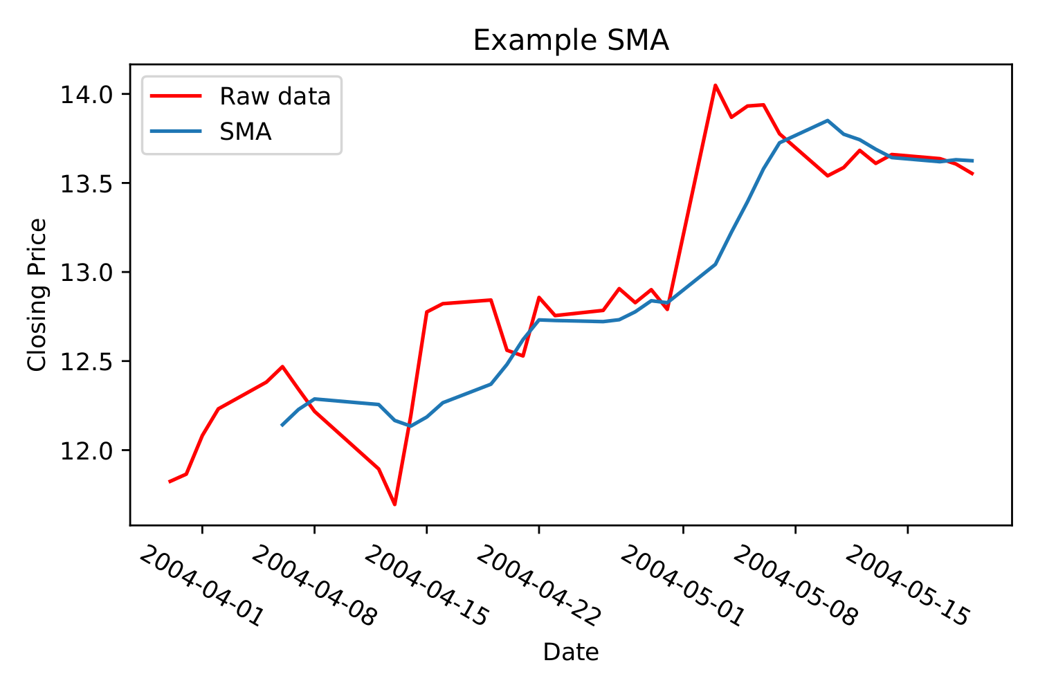
Effectively, it’s a way of smoothing out noise in the data, so we can catch trends better. The more previous data points we include, the smoother the graph. Notice, in the graph below, how the first few data points in the sma is cut off.

Exponential Moving Average (EMA)¶

Also known as EMWA - Exponentially Weighted Moving Average.

The Why¶

What we want from an ema is an indicator that, unlike a Simple Moving Average (SMA), doesn’t give equal weight to all previous data points, when depicting trends — but rather an indicator that places more trust in recent data points and less trust in more distant previous events on the timeline.

The How¶

Let’s first consider a Simple Moving Average (SMA):

\[\text{sma}_t = \dfrac{\sum\limits_{i=0}^{n} \text{price}_{(t-i)}}{n + 1}\]

If we set \(n = 3\) and abriviate price to p, starting at \(t = 3\) and looking back in time, we can expand the calculation in the following manner:

\[\dfrac{p_3 + p_2 + p_1 + p_0}{4} ~ = ~ \frac{1}{4} p_3 + \frac{1}{4} p_2 + \frac{1}{4} p_1 + \frac{1}{4} p_0\]

As we can see, the weights are equal and they sum to unity:

\[\frac{1}{4} + \frac{1}{4} + \frac{1}{4} + \frac{1}{4} ~ = ~ 1\]

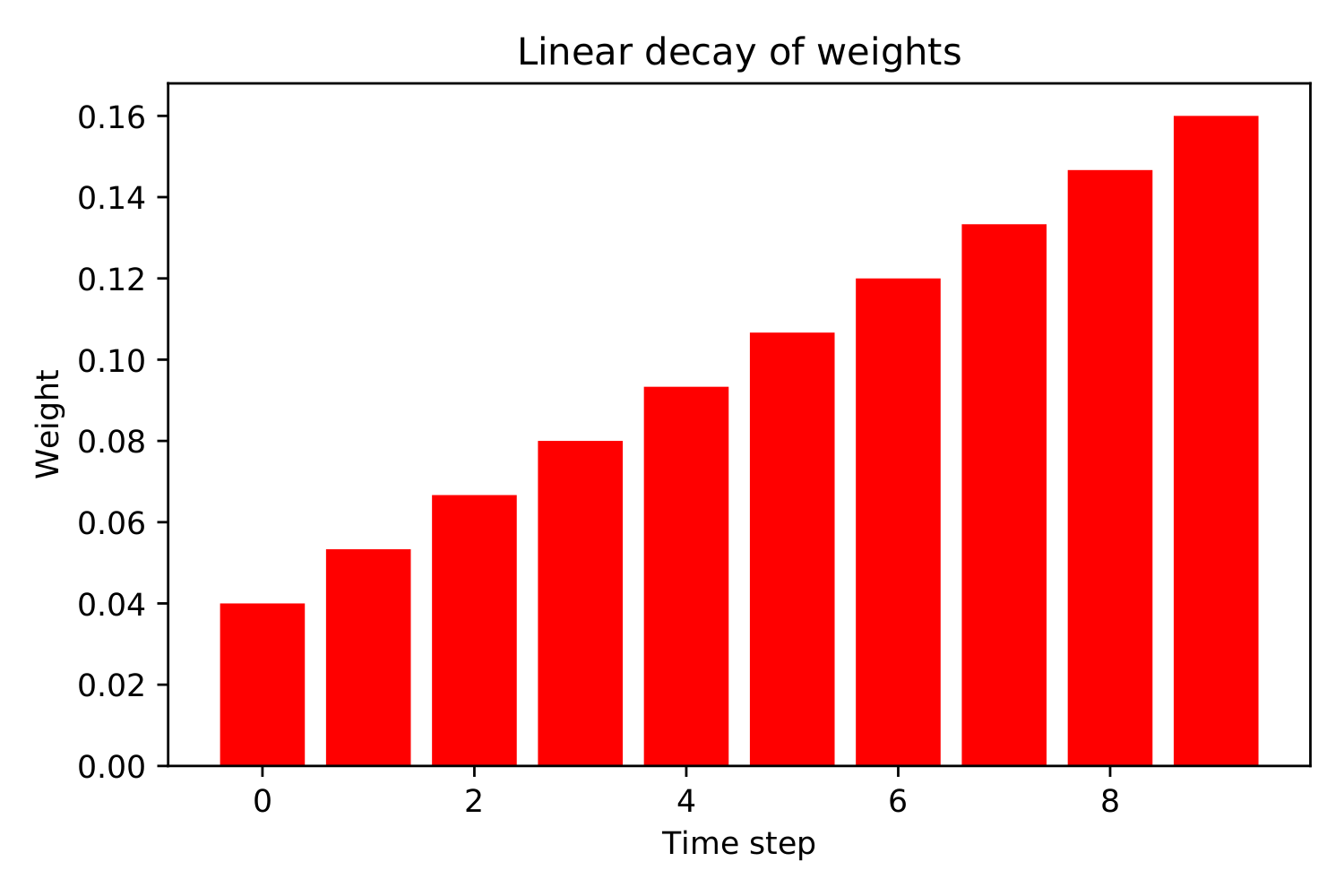
That’s integral to calculating averages. Now, if we wanted to give less weight to far gone price points, we could do reduce the weights as we go back:

\[\frac{7}{22} + \frac{6}{22} + \frac{5}{22} + \frac{4}{22} ~ = ~ 1\]

This represents a backwards linear decay of the weights for the price points. Here’s what that could look like:

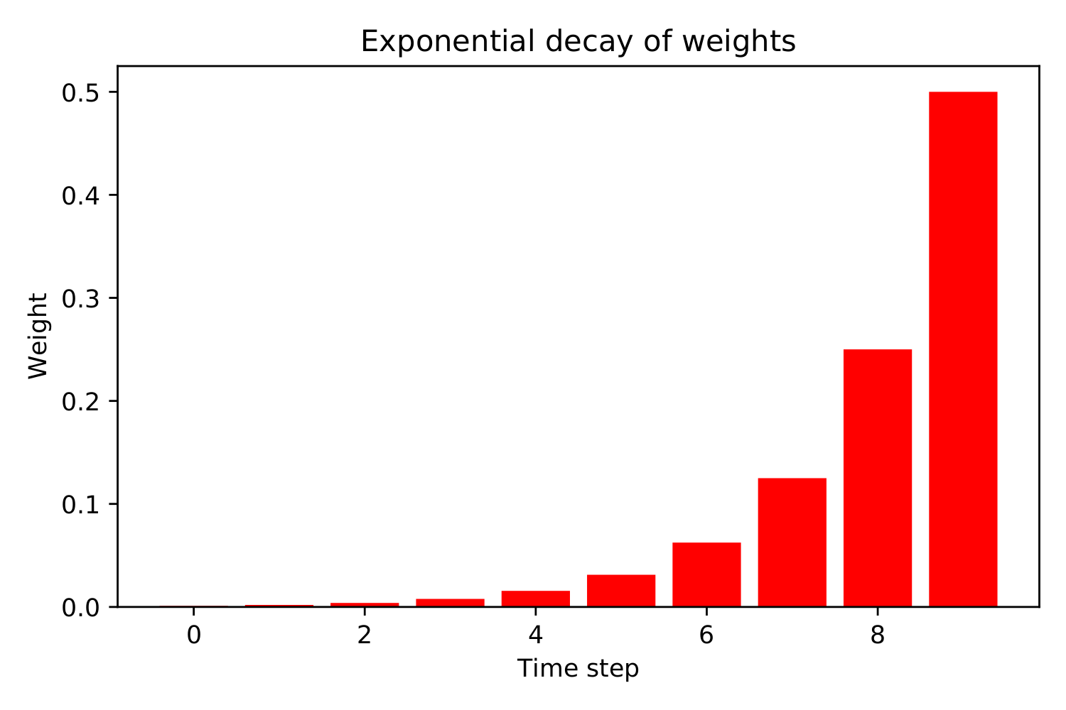
If we wanted to introduce a bit of curve to the decay, so the weights would decrease more rapidly, perhaps we could do something like:

\[\frac{1}{2} + \frac{1}{4} + \frac{1}{8} + \frac{1}{16} ~ = ~ 0.875 ~ \approx ~ 1\]

Now, \(0.875\) is not quite unity, but if keep cutting the last term in half and adding it, we quickly get very close to \(1\) — and in the limit — we get there. We can check that by adding more and more terms, or we can take the limit of a handy formula for geometric type series, like the one we just conjured up.

To see where

\[a + ar + ar^2 + \cdots + ar^{n-1},\]

is headed as \(n \rightarrow \infty\), we can use

\[\lim_{n \rightarrow \infty} \sum\limits_{i=0}^{n-1} ar^i ~ = ~ \lim_{n \rightarrow \infty} ~ a \left( \dfrac{1 - r^n}{1 - r} \right)\]

As we can see, \(a\) represents the first term in the series. In our case, that would be \(\frac{1}{2}\). The \(r\), is the common ratio — or the change each new term represents, in relation to the previous term. In our case, each new term is halved, so \(r = \frac{1}{2}\) also. So,

\[\lim_{n \rightarrow \infty} ~ \frac{1}{2} \left( \dfrac{1 - (\frac{1}{2})^{\infty}}{1 - \frac{1}{2}} \right) ~ = ~ \frac{1}{2} \left(\dfrac{1}{1 - \frac{1}{2}} \right) ~ = ~ \dfrac{\frac{1}{2}}{\frac{1}{2}} ~ = ~ 1\]

However, this only applies when \(a = (1 - r)\). If, for example, we set \(a = \frac{1}{3}\) and keep the \(r\), we do not converge to unity:

\[\frac{1}{3} \left(\dfrac{1}{1 - \frac{1}{2}} \right) ~ = ~ \dfrac{\frac{1}{3}}{\frac{1}{2}} ~ = ~ \frac{2}{3}\]

So, in order to have more freedom in setting our weights, we need to be clever about it. What we want is for

\[ \begin{align}\begin{aligned}\lim_{n \rightarrow \infty} ~ a \left( \dfrac{1 - r^n}{1 - r} \right) = 1\\\Rightarrow ~ a \left( \dfrac{1}{1 - r} \right) = 1\\\Rightarrow \dfrac{a}{1 - r} = 1\\\Rightarrow r = 1 - a\end{aligned}\end{align} \]

What that gives us is a series that look like this:

\[a + a(1 - a) + a(1 - a)^2 + a(1 - a)^3 + ~ \cdots ~ + a(1 - a)^{n-1}\]

Now, this being an infinite series, we know that we have to push \(n \rightarrow \infty\), in order to converge at unity, though it doesn’t take a very large \(n\) before we’re getting close. In our original example with \(a = r = \frac{1}{2}\) We’re already at \(0.99\) with \(7\) terms in the series sum. We’ve now finally found a way to create weights with a rapidly decreasing curve:

On top of that, we’ve pretty much derived the formula for exponential moving averages — \(p\) again short for price:

\[\text{ema}_t = \lim_{n \rightarrow \infty} \left[a p_t + a(1 - a)p_{t-1} + a(1 - a)^2p_{t-2} + ~ \cdots ~ + a(1 - a)^{n-1}p_{t-(n-1)} \right]\]

or, factoring out \(a\),

\[\text{ema}_t = \lim_{n \rightarrow \infty} ~ a \left[ p_t + (1 - a)p_{t-1} + (1 - a)^2p_{t-2} + ~ \cdots ~ + (1 - a)^{n-1}p_{t-(n-1)} \right]\]

We can express the exact same thing as a recurrent function:

\[\text{ema}_t = a p_t + (1 - a) \text{ema}_{t - 1}\]

I know, I know — recurrent functions, infinity — it can all be a bit of a mind f%!#. It might be more clear if we take the time to write out two previous timesteps:

\[ \begin{align}\begin{aligned}\text{ema}_{t-1} = a p_{t-1} + (1 - a) \text{ema}_{t - 2}\\\text{ema}_{t-2} = a p_{t-2} + (1 - a) \text{ema}_{t - 3},\end{aligned}\end{align} \]

and then substitute back into the last timestep:

\[\text{ema}_t = a p_t + (1 - a) \bigg\{ a p_{t-1} + (1 - a) \Big[ a p_{t-2} + (1 - a) \text{ema}_{t - 3} \Big] \bigg\}\]

Rewriting it, we can get:

\[ \begin{align}\begin{aligned}a p_t + a(1 - a) p_{t-1} + a(1 - a)^2 p_{t-2} + (1 - a)^3 \text{ema}_{t-3}\\a \Big[ p_t + (1 - a) p_{t-1} + (1 - a)^2 p_{t-2} \Big] + (1 - a)^3 \text{ema}_{t-3}\end{aligned}\end{align} \]

If we continued to unpack \(\text{ema}_{t-3, 4, \cdots}\), we’d eventually get back to

\[a \left[ p_t + (1 - a)p_{t-1} + (1 - a)^2p_{t-2} + ~ \cdots ~ + (1 - a)^{n-1}p_{t-(n-1)} \right],\]

if we could allow \(n \rightarrow \infty\). As we can see from the formula:

\[\text{ema}_t = a p_t + (1 - a) \text{ema}_{t - 1},\]

we always depend, ad infinitum, on the previous ema value, to calculate the current value. Our data sets, however, are never infinite, so eventually we get to \(t = 0\). Our only choice then, is to initialize \(\text{ema}_{t=0} = 0\) or approximate it somehow. We can set \(\text{ema}_{t=0} = p_{t=0}\), or scoot forward a bit and do \(\text{ema}_{t=k} = \text{sma}_{t=k}, n_{sma} = k - 1\). See Simple Moving Average (SMA). For the most part, how to initialize \(\text{ema}_{t=0}\), is not that great a concern, unless your data set is really small.

Now, one last thing: How do you choose an \(a\)? Any \(a \in (0, 1)\) can be used, but as a matter of convention — the following will do nicely:

\[a = \dfrac{2}{n_{sma} + 1}\]

If you set \(n_{sma} = 12\) in the above formula, you get what is referred to as a 12 - period EMA. Of course, as we have seen in this section, mathematically speaking, EMAs don’t have periods. They are created from approximations of infinite series. What we can say, is that with an \(a\) defined in this way, within the \(n_{sma} + 1\) first terms in the approximation of the infinite series sum, about 88% of the EMA is accounted for. Why this percentage has been chosen to represent an \(n_{sma}\) period EMA is, as of yet, unknown to us.

How to read and understand EMAs¶

When the overall slope of the EMA is rising, the EMA can serve as support. Buy when prices reach down to and below the EMA and place a protective stop somewhere below where it turns up again. Be sure to move stop as prices rice, to limit risk.
When the overall slope of the EMA is falling, the EMA can serve as resistance. Sell short when prices reach up to and beyond the EMA and place protective stop above where it turns down again. Be sure to move stop as prices fall, to limit risk.
When the market goes sideways with no apparent trend, use oscillators and not trend-following indicators, such as EMA.

Moving Average Convergence Divergence (MACD)¶

It’s commonplace to use EMAs to analyze market trends. It is, however, not a very sensitive indicator. MACD, or Moving Average Convergence Divergence, uses the difference between two EMAs to create a more sensitive indicator. A MACD indicator usually consists of two lines, a fast line, a signal line and a histogram. The fast line is the difference between two EMAs of closing prices, usually EMAs with \(n_{sma} = 12\) and \(n_{sma} = 26\) - often referred to as a 12 -and a 26 period EMA, though mathematically speaking, EMAs don’t really have periods. They are created from approximations of infinite series, as explained in the section on Exponential Moving Average (EMA). The signal line is an EMA of the fast line, usually with \(n_{sma} = 9\) and the histogram is simply the difference between the fast line and the signal line. So there you have it:

\[\begin{split}\begin{align} \mathit{MACD}_{fast} &= \mathit{EMA}_{12} - \mathit{EMA}_{26} \\ \mathit{MACD}_{signal} &= \mathit{EMA}_{9}(\mathit{MACD}_{fast}) \\ \mathit{MACD}_{histogram} &= \mathit{MACD}_{fast} - \mathit{MACD}_{signal} \end{align}\end{split}\]

How to read MACD¶

When the fast line crosses over the signal line a bullish trend is likely ahead. Buy long and place stop below latest bottom.
When the fast line crosses below the signal line a bearish trend is likely ahead. Buy long and place stop below latest top.
The MACD histogram also gives buy and sell signals, but is better for long term charts, like weekly charts. On daily charts buy signals come flying left and right. MACD histogram is actually an oscillator, but we include it here as a matter of heritage. It’s so closely linked to the MACD fast -and signal line.
- Buy when histogram stops falling and starts rising. Place stop below last bottom.
- Sell short when histogram stops rising and starts falling. Place stop above last top.
- A three month record high histogram, signals prices are likely to rise even higher.
- A three month record low histogram, signals prices are likely to fall even lower.
- A new histogram high during uptrend signals good uptrend health.
- A new histogram low during downtrend signals good downtrend health.
- Price going one way and MACD histogram the other, signals a trend is not as strong as it seems, e.g prices go up but histogram falls.

Oscillators¶

We spot trends with such indicators as Moving Average Convergence Divergence (MACD) or Exponential Moving Average (EMA). For catching turning points we turn to oscillators. Oscillators tend to catch the momentum of the market better. An oscillator oscillates between two extreme values. It’s values are derived from previous tops and bottoms. At certain levels, the market is considered oversold or overbought. They are the most accurate and useful when a trend is not very clear and the market is going sideways.